2P_line.py
Description
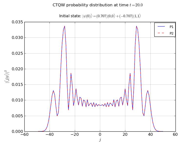
This example propagates a 2 particle continuous-time quantum walk on an infinite line
- Amongst the features used, it illustrates:
recieving command line options using PETSc
- the use of the chebyshev algorithm
- setting the EigSolver tolerance, as well as the minimum eigenvalue
adding a diagonal defects to various nodes
same-node interactions between particles
creating node handles to watch the probability at specified nodes
creating entanglement handles to watch the entanglement
- various plotting abilities:
- probability vs node plots
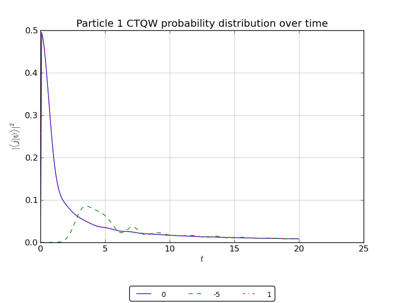
- probability vs time plots
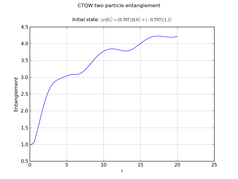
- entanglement vs time plot
Exporting the final state to a PETSc binary vector file
Source Code
1 2 3 4 5 6 7 8 9 10 11 12 13 14 15 16 17 18 19 20 21 22 23 24 25 26 27 28 29 30 31 32 33 34 35 36 37 38 39 40 41 42 43 44 45 46 47 48 49 50 51 52 53 54 55 56 57 58 59 60 61 | #!/usr/bin/env python2.7
# initialize PETSc
import sys, petsc4py
petsc4py.init(sys.argv)
from petsc4py import PETSc
import numpy as np
# import pyCTQW as qw
import pyCTQW.MPI as qw
# enable command line arguments -t and -N
OptDB = PETSc.Options()
N = OptDB.getInt('N', 100)
t = OptDB.getReal('t', 20)
# get the MPI rank
rank = PETSc.Comm.Get_rank(PETSc.COMM_WORLD)
if rank == 0:
print '2P Line\n'
# initialise an N (default 100) node graph CTQW
walk = qw.Line2P(N)
# Create a Hamiltonian with 2P interaction.
walk.createH(interaction=1.)
# create the initial state (1/sqrt(2)) (|0,0>-|1,1>)
init_state = [[0,0,1.0/np.sqrt(2.0)], [1,1,-1.0/np.sqrt(2.0)]]
walk.createInitState(init_state)
# set the eigensolver properties.
walk.EigSolver.setEigSolver(tol=1.e-2)
# underestimate the minimum eigenvalue
walk.EigSolver.setEigSolver(emin_estimate=0)
# create a handle to watch the probability at nodes -5,0,1:
walk.watch([0,1,-5])
# create a handler to watch the entanglement
walk.watch(None,watchtype='entanglement',verbose=False)
# Propagate the CTQW using the Chebyshev method
# for t=100s in timesteps of dt=0.1
for i in np.arange(0.1,t+0.1,0.1):
walk.propagate(i,method='chebyshev')
# plot the marginal probabilities
# after propagation over all nodes
walk.plot('out/2p_line_plot.png')
# plot the probability over time for the watched nodes
walk.plotNodes('out/2p_line_nodes.png')
# plot the entanglement over time
walk.plotEntanglement('out/2p_line_ent.png')
# export the final state
walk.exportState('out/2p_line_state.bin','bin')
# destroy the quantum walk
walk.destroy()
|