#!/usr/bin/env python2.7
# initialize PETSc
import sys, petsc4py
petsc4py.init(sys.argv)
from petsc4py import PETSc
import numpy as np
# import pyCTQW as qw
import pyCTQW.MPI as qw
# enable command line arguments -t and -N
OptDB = PETSc.Options()
N = OptDB.getInt('N', 10)
t = OptDB.getReal('t', 5)
# get the MPI rank
rank = PETSc.Comm.Get_rank(PETSc.COMM_WORLD)
if rank == 0:
print '3P 3-cayley Tree CTQW\n'
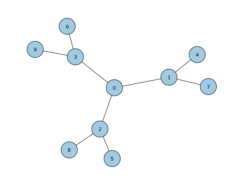
# initialise a 10 node graph CTQW
walk = qw.Graph3P(N)
# Create a 3 particle interacting Hamiltonian from a file.
# A defect of amplitude 2 and 0.5 has
# been added to nodes 3 and 4 respectively.
d = [3,4]
amp = [2.0,1.5]
walk.createH('../graphs/cayley/3-cayley.txt','txt',d=d,amp=amp,layout='spring',interaction=1.5)
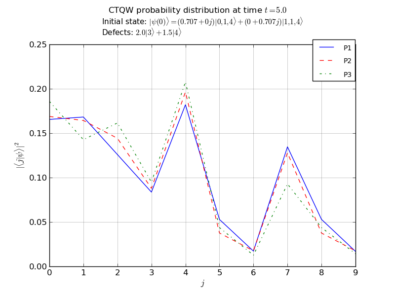
# create the initial state (1/sqrt(2)) (|0,1,4>+i|1,1,4>)
init_state = [[0,1,4,1.0/np.sqrt(2.0)], [1,1,4,1.j/np.sqrt(2.0)]]
walk.createInitState(init_state)
# set the eigensolver properties.
#Note that Emin has been set exactly.
walk.EigSolver.setEigSolver(tol=1.e-2,verbose=False,emin_estimate=0.)
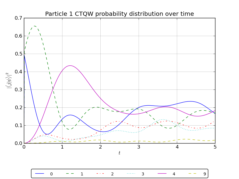
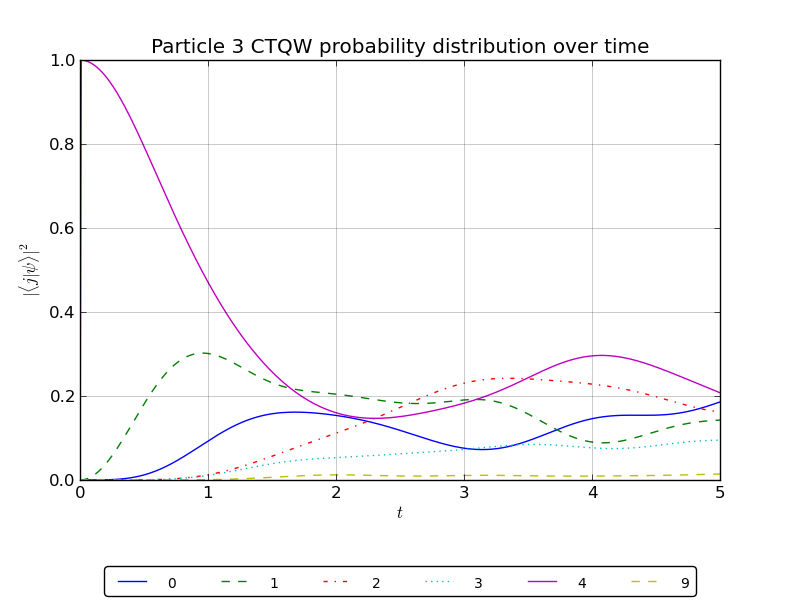
# create a handle to watch the probability at nodes 0-4,9:
walk.watch([0,1,2,3,4,9])
# Propagate the CTQW using the Chebyshev method
# for t=5s in timesteps of dt=0.01
for dt in np.arange(0.01,t+0.01,0.01):
walk.propagate(dt,method='chebyshev')
# plot the p1, p2, p3 marginal probabilities
# after propagation over all nodes
walk.plot('out/3p_3cayley_plot.png')
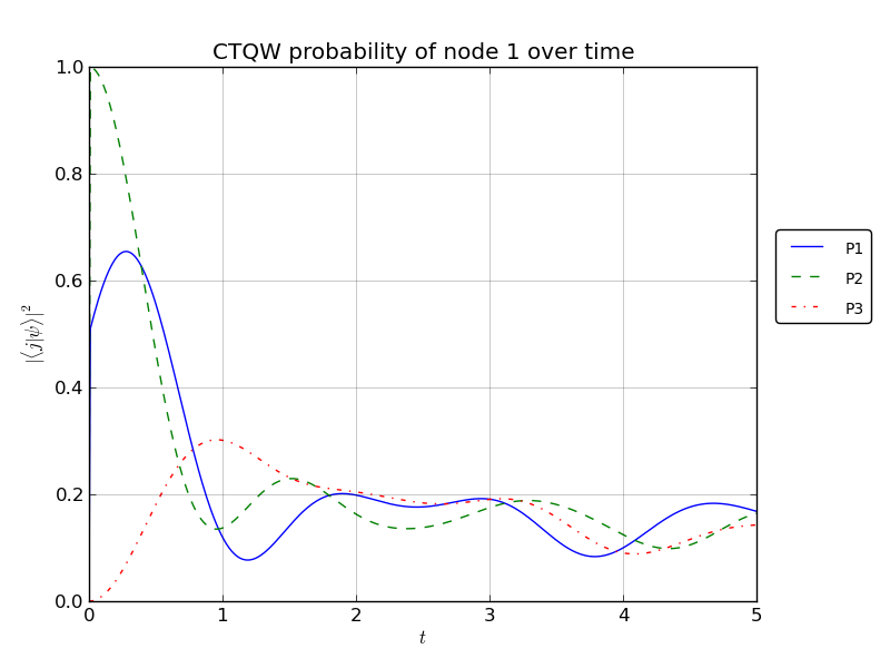
# plot the p1, p2, p3 probability over time for watched node1
walk.plotNode('out/3p_3cayley_node1.png',1)
# plot the particle 1 probability over all watched nodes
walk.plotNodes('out/3p_3cayley_nodes_particle1.png',p=1)
# plot the particle 2 probability over all watched nodes
walk.plotNodes('out/2p_3cayley_nodes_particle2.png',p=2)
# plot the particle 3 probability over all watched nodes
walk.plotNodes('out/3p_3cayley_nodes_particle3.png',p=3)
# destroy the quantum walk
walk.destroy()